EPISTOLARY PURGATORY

I spent good amount of the time between Halloween and Christmas trying to write computer programs that analyze music to pick up very specific kinds of information from them. This also perfectly fit in with a class I was taking in the Music Technology department at NYU. A problem that I was tackling towards the end of the class, was to track beats in a piece of music that varies in tempo from time to time. Like this, for example.

Humans do this remarkably well — if only we knew how.

It is worth remembering that beat tracking, or tempo detection, is a problem that is very similar to pitch detection; both try to understand change in energy with time. While pitch-detection looks at it in a very granular level to look at activity happening within a second of music, beat-detection zooms out a bit. Working on this led me to this paper on what is called Fan Chirp Transform, a special kind of transformation that involves drumroll time-warping. This blog post is all about it.

Introduction

To define this again, formally, music and audio signals are usually non-stationary in nature and it is this non-stationary aspect that is of highest interest while extracting information. So it is important to have a visual representation that not only shows frequency/spectral content in audio, but also how it changes with time.

Time-frequency representations are specially useful in two cases:

1. To look for significant temporal or spectral events so as to detect/enhance/classify the given audio
2. To work towards obtaining a sparse representation(trim out redundancies as much as possible) in this form, which is a staple method in case of audio compression. Think: How is that Radiohead song only 6MB?

The most commonly used time-frequency analysis method is the Short Term Fourier Transform (STFT). However, STFT assumes that the signal being analyzed is stationary within the analysis window, which is almost never the case for music.

This creates a trade-off between time and frequency resolution in the final spectrogram — an accurate reading on frequency requires huge time windows, which leads to uncertainty on when these frequencies materialized, and conversely, an accurate reading on events in time may lead to blurring on which exact frequencies constitute the musical event.

This is not really surprising, since, given a window of audio from a larger piece of music, it is realistic to assume that the signal rises or falls in frequencies over the course of this window. If you lazily plotted the pitch, you would still notice the rise/fall. This collective rise/fall can be characterized as the simultaneous rise/fall of lots of frequencies that make up the pitch. Each of those is called a Chirp.

If a signal started at 50Hz and rose all the way to 300Hz within a given window, an STFT would show that all the frequencies between 50 and 300Hz are present all the time. Which is not true.

There must be a way to pick up on the Chirps.

The Fan Chirp Transform (FChT) provides both time and frequency resolution using its nifty set of different chirp parameters (put together they look like a fan) as an additional dimension besides time and frequency. It is basically carried out by time-warping the signal in time domain and then using the FFT. This allows quick changes in frequency to be represented as time-traveling sinusoids.

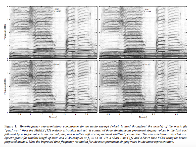
A picture from the paper that shows frequencies rising and falling with time, and how good a job various transforms do at representing it. Worth making a Joy Division t-shirt from these charts.

Math

Fan Chirp Transform is defined as:

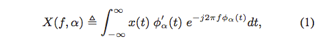
where φα(t) = (1 + (1 /2) αt)t, is a time warping function.

When the variable change τ = φα(t) is done, the formulation becomes,

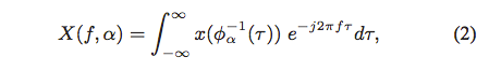
which can be considered the Fourier Transform of a time-warped signal x(t).

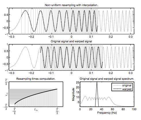
What time-warping really means here is to slow down time so that the changing frequency evens out to look like constant frequency. This is done by taking taking uniformly spaced instances of the signal and spacing them non-uniformly. The α defines how these signal instances are rearranged. Hence, the extent to which a signal rises/falls in frequencies can now be seen as the extent to which time needs to be sped up or slowed down to turn the chirp into a sinusoid.

In a digital system, FChT is performed by applying DFT to a time warped signal. The warping is done as follows:

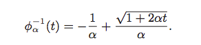
The warping function transforms linear chirps of instantaneous frequency ν(t) = (1 + αt) f into constant sinusoids of frequency ν˘(t) = f. In a practical implementation, the original signal is processed in short time frames where each analysis window is centered with respect to the constant sinusoid. Which means, for the 50–300Hz example, the window will be centered somewhere around 180Hz or so.

Letting Math help twist time so everything moves in the same speed. Changes in frequency can now be represented as ‘how much time warping do we need here?’

Pitch Salience

The goal of pitch salience computation is to build a continuous function that gives a prominence value for each fundamental frequency in a certain range of interest. This allows you to look at every analysis window as a snapshot in time and not only know what frequencies are present in it, but also what happened to them by the end of the window.

In the real world (where music happens), objects don’t make sounds in just one frequency. They almost always give out additional harmonics that are either multiples or submultiples of the fundamental frequencies. What you hear is the sum of all of these. Which is why a C# sounds different on a piano and a guitar. They give out different harmonics.

In order to avoid spurious peaks at these multiples and submultiples, a common approach for pitch salience calculation is to define a fundamental frequency grid, and compute for each frequency, a weighted sum of the partial amplitudes.

Since the values of α(time-warp parameter) used in the analysis are discrete, if a chirp rate does not closely match any of the available α values, higher partials continue to behave non-stationarily after the time-warping, threatening to defeat purpose. Using the CQT alleviates this problem. I am not entirely sure how CQT works but my wild guess is that it does some kind of interpolation. Maybe I’ll read up on it sometime.

Zooming Out, Into Context

The reason I even began reading this paper was because a friend and I wanted to find a way of using pitch-detection algorithms to detect beats. However for this, a bunch of other things need to be done. An important step there is to extract what is called the Novelty Function, which takes a piece of music and gives you only a function of its loudness. This does away with frequency content, and looks at other periodically occurring events — like a beat. The FChT is applied to this and then the resulting tempo-salience(in my case) is used as fodder for a machine learning algorithm that likes to pretend music is a Markov chain. I’m still in the process of figuring out if we’re onto something cool here.

The Fan Chirp Transform really serves as a cog in my project, but you have to admit — it is interesting that you can control time with math.