EPISTOLARY PURGATORY

I looked far and wide for material to understand the Experts Advice framework for a machine learning class at school. A lot of it is lecture slides and papers, both being obtuse and inaccessible in their own way. I ended up parsing through slides and wrapping my head around some of the math. I figured I should put it here so you can save yourself the effort. There is some amount of basic probability knowledge that I am taking for granted. That stuff is worth knowing in general.

I’ve tried my best to make the math and notations as clear and pretty as possible.

Experts Advice is an online machine learning framework that learns from its mistakes over time and tries to predict things into the future. While all of machine learning pretty much revolves around creatively punishing a computer for its mistakes, experts advice operates in a more meta realm: The system does not make its own calculated prediction, but merely processes the combined prediction of a bunch of experts. It also incurs the loss of making a bad prediction and uses it to prioritize one expert over the other.

For the purpose of this discussion, let us treat each of these experts as a black box — they happen to predict alright for some reason, but they also go wrong every now and then. We do not know how good any of them is.

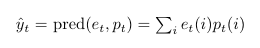
The goal for the learner is to be able to accurately predict the outcome at any time t. The learner keeps account of a distribution pt, which is the probability distribution of the experts to make the correct prediction at that time t. We will need this distribution to change with time, as it dictates which expert deserves to be given how much importance, or weightage. pt(i) denotes the probability that the ith expert will predict correctly at time t. If this value is high, the expert will be taken seriously. If it’s low, too bad.

The learner takes all these individual predictions(et’s) to make a final prediction informed by all of them. This is denoted by:

Based on the real outcome, the learner incurs its loss and updates pt to reflect which experts are more likely to get the next one right. It’s almost a reverse betting game.

Loss Functions

In an experts advice framework, the loss is also a function of time. The loss accumulated at the end of a certain period of time is called regret. We will use these loss functions when the time is right. But it’s worth defining notations and basic ideas beforehand.

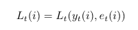
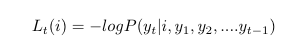
The loss of an expert i at time t is expressed as:

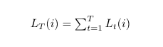
The cumulative loss of this expert i at the end of T time steps is:

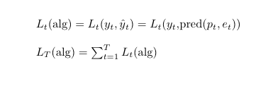
The loss incurred by the overall learning algorithm at time t and end of T time steps is:

The entire model updates its parameters at every time step, and the future prediction by the learner is almost entirely dictated by its parameters at the current time instant. It is very tempting to look at the whole learning process of the experts advice framework as a Hidden Markov Model. We will not resist this temptation.

Hidden Markov Model

The Hidden Markov Model(HMM) roughly functions in the following way: We watch a process (any process) and make a series of observations over time. The observations from one instant to another may seem to vary with no obvious connection. However, we work with a belief that there is a certain mechanism that governs this process, and that at each time instant, this mechanism exhibits a certain hidden state that results in the system to throw out what we call observations.

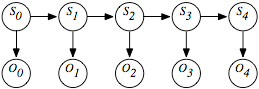
S is state. O is observation. And this image comes from here

Consider lights in a christmas decoration. The lights blink and strobe and change colors very arbitrarily — the randomness almost adds to the aesthetic. However, we all know there is a specific hidden pattern to how these lights change. There probably is a little chip somewhere near the power plug that lets current through based on a set of rules. If we stared the lights for long enough and chose to do statistics on it (both are very bad ideas for Christmas), we could roughly come up with a string of hidden rules that the little chip plays by to get the christmas lights running.

Let’s fantasize further and pretend this christmas light chip has a hint of randomization in its rules. This means that its shift from one step to another can be defined by a transition probability. Given a state (or the observations it causes) and the transition probability, we could make a good guess on what the lights will do next.

Adapting HMM to Experts Advice

In adapting the HMM to experts advice, here are a few relations we should establish.

1. The hidden state is the identity of the best expert at a given time instant t.
2. The observation is the actual outcome yt.
3. The transition probability will be a matrix of probability values that tell who is more likely to be the best expert in the next time instant, given we know the current one.

Now, consider this: in the real world, things are chaotic. So a given state doesn’t necessarily have to result in the same observation every time. Or multiple states may end up causing the same observation at different times. So we also factor a probability here called the emission probability that gives you how likely it is that a given observation was emitted by some hidden state i of all states. Or in our case, it is the probability that the ith expert was given the highest weightage during the current prediction.

If the current prediction went great, the learner may pat itself on the back and take the same expert more seriously by increasing weights for it. If the prediction was wrong, the learner will have to start getting wary of the ith expert and reduce its weights. Either way, the emission probability is what helps the learner learn from its mistakes. We will hence base our loss function on it.

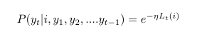
ƞ is the acceleration constant that speeds up/slows down the learning process.

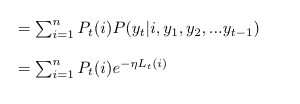
Let’s also define the probability of a given outcome, given past outcomes. This will be:

∑ (Probability of current best expert).(Emission prob. for current outcome)

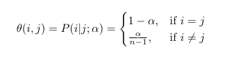
Remember the hidden state is the identity of best expert. So the transition probability matrix gives information about the tendency of the ‘best expert’ title to get passed on to someone else. We characterize this using the constant, ɑ. As ɑ gets higher, the ‘best expert’ title switches more frequently. This may or may not be a good thing. Nevertheless, our transition probability (*Θ)* is defined as

Now that we know a way to penalize the learner for its mistakes as well as watch change in best expert with time, we can build our update function by putting these probabilities together. The rule for updating pt, having decided on an ɑ is:

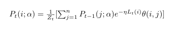
It looks crazy but it isn’t. It’s just the product of previous weight, the loss that came with it, and the transition probability to current weight for each expert, all summed up.

Zt is a normalizing factor to make sure pt is always between 0 and 1.

By tweaking with ɑ, we can build two different kinds of expert advice based learners.

1. By setting ɑ to 0, we get a system that never lets go once it gets hold of a best expert. This framework is called the static expert framework. The learner starts with equal weightage to all experts, but as soon as it narrows in on one best expert, it progressively increases weights for that one while burying everything else. This is useful if all we want to do is find which expert does the job well.
2. When ɑ is kept a constant, it freezes the tendency for the best expert to keep changing. In other words, it makes sure that every expert gets an equal share of the loss incurred by the learner, regardless of how well each of them did. This framework is called the fixed share. This is useful when each expert is good at predicting at different situations(using different features) and we need to keep them all around. This way if one expert temporarily fails, the others will compensate for the error.

I stop here. But there is so much more research and literature out there that deals with the various ways you can tweak the transition probabilities, or theoretically derive the worst case regret in order to get a hang of how bad the learner can possibly get, given a set of experts. There is also an interesting learn-ɑ algorithm that is another machine learning algorithm on top of this one, which picks the best ɑ from time to time to make sure the system learns fine.

The equations here aren’t too hard to code and prototype on something like MATLAB. NumPy is a probably better idea. Coding helps in understanding this more clearly.

If math doesn’t bother you, this is probably a paper you will like. That’s a big if, but I will leave that to your judgement.